Hands-On Guide to Time Series Analysis using Simple Exponential Smoothing in Python

A time series tracks the movement of the datapoint over a period of time. Usually, Time-series depicts the value of data at equal intervals of time.  Data related to stocks, depreciation of machinery, insurance premium, etc. can be considered as Time series data as it tends to change from time to time. Time series is a part of our everyday life. 

In this article, we will explore:

• Time Series Analysis
• Simple Exponential Smoothing
• Time series forecasting using Simple Exponential Smoothing

Through the Simple Exponential smoothing model, we will analyze a time series and infer the predictions through this.

Time Series Analysis

Time series analysis is studying a particular time series over a particular time period to observe any pattern which can be used to predict future values for that time series. Whether it is analyzing the stock data for the previous year or analyzing the sales of a company over a period of time, etc. all this comes under Time Series Analysis and Prediction. For more understanding, you can refer to our articles “An Introductory Guide to Time Series Forecasting” and “Understanding Time Series Analysis: A Deep Dive”.

Simple Exponential Smoothing

Simple Exponential Smoothing is used for time series prediction when the data particularly  does not follow any:

1. Trend: An upward or downward slope
2. Seasonality: Shows a particular pattern due to seasonal factors like Hours, days, Year, etc.

SES works on weighted averages i.e. the average of the previous level and current observation. The largest weights are associated with the recent observations and the smallest weights are associated with the oldest observations.

The decrease in weight is controlled by the smoothing parameter which is known as ???? (alpha) here. ????(alpha) value can be between 0 to 1:

• ????(alpha)=0: Means that forecast for future value is the average of historical data.
• ????(alpha)=1: Means that forecast for all future value is the value of the last observation    

• How To Apply Smoothing Methods In Time Series Analysis
• Beginners Guide To Linear Regression In Python
• Top 8 Data Transformation Methods
• The New Face of War: AI-driven Drones
• Job Alert: 5 Current Openings For ML Engineers In India

Time series forecasting using Simple Exponential Smoothing in Python

Simple Exponential Smoothing (SES) is defined under the statsmodel library of python and like any other python library we can install statsmodel using pip install statsmodel.

a. Importing the required libraries

Simple Exponential Smoothing is defined under the statsmodel library from where we will import it. We will import pandas also for all mathematical computations.

import pandas as pd
from statsmodels.tsa.api import SimpleExpSmoothing

b. Loading the dataset

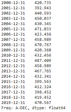
Simple exponential smoothing works best when there are fewer data points. Here I have created a fake dataset that we can observe as the sales data of a company from the year 2000 to 2019.  We will create the dataset as given below.

df = [ 420.735,392.943, 440.593, 450.037, 430.345, 471.033, 423.456, 458.989, 470.767, 420.368, 432.456, 487.409, 458.989, 467.765, 432.341, 399.563, 412.324, 398.452, 419.452, 470.567]

c.Creating a time series of the data

To visualize and analyze the sales data let us create a time series of this fake dataset. The frequency of the time series is annually so we will pass the argument “A” in the series function.

index= pd.date_range(start='2000', end='2020', freq='A')
data = pd.Series(df, index)
print(data)

d. Visualize the Data

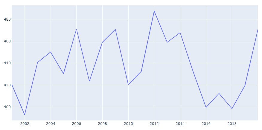
Now we will analyze this data using a line chart. We will use the Plotly library for visualization.

import plotly.express as px
fig = px.line(data)
fig.show()

The data clearly shows that there is no particular trend or seasonality in sales. So choosing this type of data is better for prediction using Simple Exponential Smoothing.

e. Prediction using SES

For creating a prediction model using SES we should have a ????(alpha) value which we discussed in the beginning. Here we will create three instances in which we will take three different ????(alpha) values as:

1. ????(alpha) = 0.2
2. ????(alpha) = 0.8
3. ????(alpha) value automatically optimized by statsmodel which is the recommended one.

We will pass the data into Simple Exponential Smoothing and fit the data with different values of the Smoothing Level.

#First Instance
ins1 = SimpleExpSmoothing(data).fit(smoothing_level=0.2,optimized=False)
ins_cast1 = ins1.forecast(3).rename('alpha=0.2')

#Second Instance
ins2 = SimpleExpSmoothing(data).fit(smoothing_level=0.8,optimized=False)
ins_cast2 = ins2.forecast(3).rename('alpha=0.8')

#Third Instance
ins3 = SimpleExpSmoothing(data).fit()
ins_cast3 = ins3.forecast(3).rename('alpha=%s'%ins3.model.params['smoothing_level'])

#After creating model we will visualize the plot
ax = data.plot(marker='o', color='black', figsize=(12,8), legend=True)

#Plot for alpha =0.2
ins_cast1.plot(marker='+', ax=ax, color='blue', legend=True)
ins1.fittedvalues.plot(marker='+', ax=ax, color='blue')

#Plot for alpha = 0.8
ins_cast2.plot(marker='o', ax=ax, color='red', legend=True)
ins2.fittedvalues.plot(marker='o', ax=ax, color='red')

#Plot for alpha=Optimized by statsmodel
ins_cast3.plot(marker='*', ax=ax, color='green', legend=True)
ins3.fittedvalues.plot(marker='*', ax=ax, color='green')

plt.show()

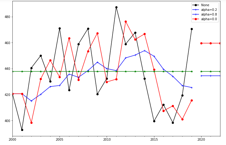
In this plot, we can see that the black line is the actual distribution of the data, other than that the red line plot is the most accurate as it is plotted according to the optimized value determined by the statsmodel itself. 

Here we can also see that the optimized value of the smoothing level predicts the value of sales for the next year that it will be around 460 which seems to be possible.

Other than Simple Exponential Smoothing there are many other Exponential Smoothing models that work for time series prediction, namely:

1. Holt’s Method: This method is used when the data shows a particular trend like an upward or a downward slope. Here we have two smoothing equations one for level and the other one for trend.
2. Holt’s Winter Method:  This method is used when data has a certain trend and seasonality also for eg. data shows an upward trend and that too in a particular month. Similar to the other exponential smoothing methods it has smoothing parameters like level, Trend. Also, a third parameter seasonality is also added in this model. 

Conclusion

In this article, we saw what is a time series and how it looks. We learned about a time Series prediction Model named Simple Exponential Smoothing which works on Time Series data which has no particular trend or seasonality. We also visualized the prediction of the model through which we could infer the predicted value.